Measurements are an integral part of living; we measure time, measure steps walked to know the calories burnt, measure the materials added for cooking, and measure the size of clothes to know whether it fits perfectly. Sometimes we fail to know the exact measurement, and the values vary, leading to errors. In this article, let us learn about measurement, errors in measurement, types of errors and how to avoid the errors.
Table of Contents:
-
- Measurement
- Types of Errors
- Errors Calculation
- How To Reduce Errors In Measurement
- Frequently Asked Questions – FAQs
Measurement is the foundation for all experimental science. All the great technological development could not have been possible without ever-increasing levels of accuracy of measurements. The measurement of an amount is based on some international standards, which are completely accurate compared with others. Just like your vegetable vendors, measurements are taken by comparing an unknown amount with a known weight. Every measurement carries a level of uncertainty which is known as an error. This error may arise in the process or due to a mistake in the experiment. So 100% accurate measurement is not possible with any method.
An error may be defined as the difference between the measured and actual values. For example, if the two operators use the same device or instrument for measurement. It is not necessary that both operators get similar results. The difference between the measurements is referred to as an ERROR.
To understand the concept of measurement errors, you should know the two terms that define the error. They are true value and measured value. The true value is impossible to find by experimental means. It may be defined as the average value of an infinite number of measured values. The measured value is a single measure of the object to be as accurate as possible.
Types of Errors
There are three types of errors that are classified based on the source they arise from; They are:
- Gross Errors
- Random Errors
- Systematic Errors
Gross Errors
This category basically takes into account human oversight and other mistakes while reading, recording, and readings. The most common human error in measurement falls under this category of measurement errors. For example, the person taking the reading from the meter of the instrument may read 23 as 28. Gross errors can be avoided by using two suitable measures, and they are written below:
- Proper care should be taken in reading, recording the data. Also, the calculation of error should be done accurately.
- By increasing the number of experimenters, we can reduce the gross errors. If each experimenter takes different readings at different points, then by taking the average of more readings, we can reduce the gross errors
Random Errors
The random errors are those errors, which occur irregularly and hence are random. These can arise due to random and unpredictable fluctuations in experimental conditions (Example: unpredictable fluctuations in temperature, voltage supply, mechanical vibrations of experimental set-ups, etc, errors by the observer taking readings, etc. For example, when the same person repeats the same observation, he may likely get different readings every time.
This article explored the various types of errors in the measurements we make. These errors are everywhere in every measurement we make. To find more articles, visit BYJU’S. Join us and fall in love with learning.
Systematic Errors:
Systematic errors can be better understood if we divide them into subgroups; They are:
- Environmental Errors
- Observational Errors
- Instrumental Errors
Environmental Errors: This type of error arises in the measurement due to the effect of the external conditions on the measurement. The external condition includes temperature, pressure, and humidity and can also include an external magnetic field. If you measure your temperature under the armpits and during the measurement, if the electricity goes out and the room gets hot, it will affect your body temperature, affecting the reading.
Observational Errors: These are the errors that arise due to an individual’s bias, lack of proper setting of the apparatus, or an individual’s carelessness in taking observations. The measurement errors also include wrong readings due to Parallax errors.
Instrumental Errors: These errors arise due to faulty construction and calibration of the measuring instruments. Such errors arise due to the hysteresis of the equipment or due to friction. Lots of the time, the equipment being used is faulty due to misuse or neglect, which changes the reading of the equipment. The zero error is a very common type of error. This error is common in devices like Vernier callipers and screw gauges. The zero error can be either positive or negative. Sometimes the scale readings are worn off, which can also lead to a bad reading.
Instrumental error takes place due to :
- An inherent constraint of devices
- Misuse of Apparatus
- Effect of Loading
Errors Calculation
Different measures of errors include:
Absolute Error
The difference between the measured value of a quantity and its actual value gives the absolute error. It is the variation between the actual values and measured values. It is given by
Absolute error = |VA-VE|
Percent Error
It is another way of expressing the error in measurement. This calculation allows us to gauge how accurate a measured value is with respect to the true value. Per cent error is given by the formula
Percentage error (%) = (VA-VE) / VE) x 100
Relative Error
The ratio of the absolute error to the accepted measurement gives the relative error. The relative error is given by the formula:
Relative Error = Absolute error / Actual value
How To Reduce Errors In Measurement
Keeping an eye on the procedure and following the below listed points can help to reduce the error.
- Make sure the formulas used for measurement are correct.
- Cross check the measured value of a quantity for improved accuracy.
- Use the instrument that has the highest precision.
- It is suggested to pilot test measuring instruments for better accuracy.
- Use multiple measures for the same construct.
- Note the measurements under controlled conditions.
Frequently Asked Questions – FAQs
What is meant by measurement error?
The difference between a measured quantity and its true value gives measurement error.
What are the types of errors?
The following are the types of errors:
- Gross Errors
- Random Errors
- Systematic Errors
The error seen due to the effect of the external conditions on the measurement is known as?
It is known as the environmental error.
Define absolute error?
Absolute error is the variation between the actual values and measured values. It is given by
Absolute error = |VA-VE|
A length was calculated to be 10.1 feet, but the absolute length was 10.5 feet. Calculate the absolute error.
We know that, Absolute error = |VA-VE|
Absolute error = 10.5-10.1 = 0.4 feet
Know in detail about absolute and relative error measurement. Visit BYJU’S – The Learning App and fall in love with learning!!

Let’s first know some basics about numbers used in floating-point arithmetic or in other words Numerical analysis and how they are calculated.
Basically, all the numbers that we use in Numerical Analysis are of two types as follows.
- Exact Numbers –
Numbers that have their exact quantity, means their value isn’t going to change. For example- 3, 2, 5, 7, 1/3, 4/5, or √2 etc. - Approximate Numbers –
These numbers are represented in decimal numbers. They have some certain degrees of accuracy. Like the value of π is 3.1416 if we want more precise value, we can write 3.14159265, but we can’t write the exact value of π.These digits that we use in any approximate value, or in other way digits which represent the numbers are called Significant Digits.
How to count significant digits in a given number :
For example –
In the normal value of π (3.1416), there are 5 significant digits and when we write more precise value of it (3.14159265) we get 9 significant digits.
Let’s say we have numbers: 0.0123, 1.2300, and 0.10234. Now we have 4, 3, and 5 significant digits respectively.
In the Scientific Representation of numbers –
2.345×10⁷, 8.7456 ×10⁴, 5.4×10⁶ have 4, 5 and 2 significant digits respectively.
Absolute Error :
Let the true value of a quantity be X and the approximate value of that quantity be X1. Hence absolute error has defined the difference between X and X1. Absolute Error is denoted by EA.
Hence EA= X-X1=δX
Relative Error :
It is defined as follow.
ER = EA/X = (Absolute Error)/X
Percentage Error :
It is defined as follow.
EP= 100×EP= 100×EA/X
Let’s say we have a number δX = |X1-X|, It is an upper limit on the magnitude of Absolute Error and known as Absolute Accuracy.
Similarly the quantity δX/ |X| or δX/ |X1| called Relative Accuracy.
Now let’s solve some examples as follows.
- Ex-1 :
We are given an approximate value of π is 22/7 = 3.1428571 and true value is 3.1415926. Calculate absolute, relative and percentage errors?
Solution –We have True value X= 3.1415926, And Approx. value X1= 3.1428571. So now we calculate Absolute error, we know that EA= X - X1=δX Hence EA= 3.1415926- 3.1428571 = -0.0012645 Answer is -0.0012645 Now for Relative error we’ve (absolute error)/(true value of quantity) Hence ER = EA/X = (Absolute Error)/X, EA=(-0.0012645)/3.1415926 = -0.000402ans. Percentage Error, EP= 100 × EA/X = 100 × (-0.000402) = - 0.0402ans.
- Ex-2 :
Let the approximate values of a number 1/3 be 0.30, 0.33, 0.34. Find out the best approximation.
Solution –
Our approach is that we first find the value of Absolute Error, and any value having the least absolute will be best. So, we first calculate the absolute errors in all approx values are given.
<pre
|X-X1| = |1/3 – 0.30| = 1/30
|1/3 – 0.33| = 1/300
|1/3 – 0.34| = 0.02/3 = 1/500Hence, we can say that 0.33 is the most precise value of 1/3;
- Ex-3 :
Finding the difference—
√5.35 - √4.35
Solution –
√5.35 = 2.31300
√4.35 = 2.08566
Hence, √5.35 - √4.35 = 2.31300 – 2.08566 = 0.22734
Here our answer has 5 significant digits we can modify them as per our requirements.
Measurement is a major part of scientific calculations. Completely accurate measurement results are absolutely rare. While measuring different parameters, slight errors are common. There are different types of errors, which cause differences in measurement. All the errors can be expressed in mathematical equations. By knowing the errors, we can calculate correctly and find out ways to correct the errors. There are mainly two types of errors – absolute and relative error. In this article, we are going to define absolute error and relative error. Here, we are giving explanations, formulas, and examples of absolute error and relative error along with the definition. The concept of error calculation is essential in measurement.
Define Absolute Error
Absolute error is defined as the difference between the actual value and the measured value of a quantity. The importance of absolute error depends on the quantity that we are measuring. If the quantity is large such as road distance, a small error in centimetres is negligible. While measuring the length of a machine part an error in centimetre is considerable. Though the errors in both cases are in centimetres, the error in the second case is more important.
Absolute Error Formula
The absolute error is calculated by the subtraction of the actual value and the measured value of a quantity. If the actual value is x₀ and the measured value is x, the absolute error is expressed as,
∆x = x₀- x
Here, ∆x is the absolute error.
Absolute Error Example
Here, we are giving an example of the absolute error in real life. Suppose, we are measuring the length of an eraser. The actual length is 35 mm and the measured length is 34.13 mm.
So, The Absolute Error = Actual Length — Measured Length
= (35 — 34.13) mm
= 0.87 mm
Classification Of Absolute Error
-
Absolute accuracy error
Absolute accuracy error is the other name of absolute error. The formula for absolute accuracy error is written as E= E exp – E true, where E is the absolute accuracy error, E exp is the experimental value and E true is the actual value.
-
Mean absolute error
MAE or the mean absolute error is the mean or average of all absolute errors. The formula for Mean Absolute Error is given as,
MAE = [frac{1}{n}] [sum_{i=1}^{n}mid x_{i} -xmid]
-
Absolute Precision Error
It is a standard deviation of a group of numbers. Standard deviation helps to know how much data is spread.
Relative Error Definition
The ratio of absolute error of the measurement and the actual value is called relative error. By calculating the relative error, we can have an idea of how good the measurement is compared to the actual size. From the relative error, we can determine the magnitude of absolute error. If the actual value is not available, the relative error can be calculated in terms of the measured value of the quantity. The relative error is dimensionless and it has no unit. It is written in percentage by multiplying it by 100.
Relative Error Formula
The relative error is calculated by the ratio of absolute error and the actual value of the quantity. If the absolute error of the measurement is ∆x, the actual value is x0, the measured value is x, the relative error is expressed as,
xᵣ = (x₀ — x)/ x₀ = ∆x/x₀
Here, xr is the relative error.
Relative Error Example
Here, we are giving an example of relative error in real life. Suppose, the actual length of an eraser is 35 mm. Now, the absolute error = (35-34.13) mm = 0.87 mm.
So, the relative error = absolute error/actual length
= 0.87/35
= 0.02485
(Image will be Uploaded Soon)
Relative Error as a Measure of Accuracy
In many cases, relative error is a measure of precision. At the same time, it can also be used as a measure of accuracy. Accuracy is the extent of knowing how accurate the value is as compared to the actual or true value. Students can find the RE accuracy only if they know the true value or measurement. For simplicity, we have the formula for calculating the RE accuracy which is given as
RE[_{accuracy}] = Actual error/ true value * 100%
Absolute Error and Relative Error in Numerical Analysis
Numerical analysis of error calculation is a vital part of the measurement. This analysis finds the actual value and the error quantity. The absolute error determines how good or bad the measurement is. In numerical calculation, the errors are caused by round-off error or truncation error.
Absolute and Relative Error Calculation — Examples
1. Find the absolute and relative errors. The actual value is 125.68 mm and the measured value is 119.66 mm.
Solution:
Absolute Error = |125.68 – 119.66| mm
= 6.02 mm
Relative Error = |125.68 – 119.66| / 125.68
= 0.0478
2. Find out the absolute and relative errors, where the actual and measured values are 252.14 mm and 249.02 mm.
Solution:
Absolute Error = |252.14 – 249.02| mm
= 3.12 mm
Relatives Error = 3.12/252.14
= 0.0123
Did You Know?
In different measurements, the quantity is measured more than one time to get an average value of the quantity. Mean absolute error is one of the most important terms in this kind of measurement. The average of all the absolute errors of the collected data is called the MAE ( Mean Absolute Error). It is calculated by dividing the sum of absolute errors by the number of errors. The formula of MAE is –
MAE = [frac{displaystylesumlimits_{i=1}^n mid x_{0}-x mid }{n}]
Here,
n is the number of errors,
x₀ is the actual value,
x is the measured value, and
|x₀-x| is the absolute error.
Absolute and Relative Error Calculation
Brand X Pictures/Getty Images
Updated on October 06, 2019
Absolute error and relative error are two types of experimental error. You’ll need to calculate both types of error in science, so it’s good to understand the difference between them and how to calculate them.
Absolute error is a measure of how far ‘off’ a measurement is from a true value or an indication of the uncertainty in a measurement. For example, if you measure the width of a book using a ruler with millimeter marks, the best you can do is measure the width of the book to the nearest millimeter. You measure the book and find it to be 75 mm. You report the absolute error in the measurement as 75 mm +/- 1 mm. The absolute error is 1 mm. Note that absolute error is reported in the same units as the measurement.
Alternatively, you may have a known or calculated value and you want to use absolute error to express how close your measurement is to the ideal value. Here absolute error is expressed as the difference between the expected and actual values.
Absolute Error = Actual Value — Measured Value
For example, if you know a procedure is supposed to yield 1.0 liters of solution and you obtain 0.9 liters of solution, your absolute error is 1.0 — 0.9 = 0.1 liters.
Relative Error
You first need to determine absolute error to calculate relative error. Relative error expresses how large the absolute error is compared with the total size of the object you are measuring. Relative error is expressed as a fraction or is multiplied by 100 and expressed as a percent.
Relative Error = Absolute Error / Known Value
For example, a driver’s speedometer says his car is going 60 miles per hour (mph) when it’s actually going 62 mph. The absolute error of his speedometer is 62 mph — 60 mph = 2 mph. The relative error of the measurement is 2 mph / 60 mph = 0.033 or 3.3%
Sources
- Hazewinkel, Michiel, ed. (2001). «Theory of Errors.» Encyclopedia of Mathematics. Springer Science+Business Media B.V. / Kluwer Academic Publishers. ISBN 978-1-55608-010-4.
- Steel, Robert G. D.; Torrie, James H. (1960). Principles and Procedures of Statistics, With Special Reference to Biological Sciences. McGraw-Hill.
From Wikipedia, the free encyclopedia
In statistics, mean absolute error (MAE) is a measure of errors between paired observations expressing the same phenomenon. Examples of Y versus X include comparisons of predicted versus observed, subsequent time versus initial time, and one technique of measurement versus an alternative technique of measurement. MAE is calculated as the sum of absolute errors divided by the sample size:[1]

It is thus an arithmetic average of the absolute errors  , where
  is the prediction and
  the true value. Note that alternative formulations may include relative frequencies as weight factors. The mean absolute error uses the same scale as the data being measured. This is known as a scale-dependent accuracy measure and therefore cannot be used to make comparisons between series using different scales.[2] The mean absolute error is a common measure of forecast error in time series analysis,[3] sometimes used in confusion with the more standard definition of mean absolute deviation. The same confusion exists more generally.
Quantity disagreement and allocation disagreement[edit]
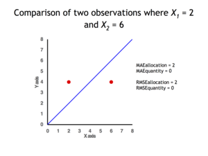
2 data points for which Quantity Disagreement is 0 and Allocation Disagreement is 2 for both MAE and RMSE
It is possible to express MAE as the sum of two components: Quantity Disagreement and Allocation Disagreement. Quantity Disagreement is the absolute value of the Mean Error given by:[4]

Allocation Disagreement is MAE minus Quantity Disagreement.
It is also possible to identify the types of difference by looking at an  plot. Quantity difference exists when the average of the X values does not equal the average of the Y values. Allocation difference exists if and only if points reside on both sides of the identity line.[4][5]
[edit]
The mean absolute error is one of a number of ways of comparing forecasts with their eventual outcomes. Well-established alternatives are the mean absolute scaled error (MASE) and the mean squared error. These all summarize performance in ways that disregard the direction of over- or under- prediction; a measure that does place emphasis on this is the mean signed difference.
Where a prediction model is to be fitted using a selected performance measure, in the sense that the least squares approach is related to the mean squared error, the equivalent for mean absolute error is least absolute deviations.
MAE is not identical to root-mean square error (RMSE), although some researchers report and interpret it that way. MAE is conceptually simpler and also easier to interpret than RMSE: it is simply the average absolute vertical or horizontal distance between each point in a scatter plot and the Y=X line. In other words, MAE is the average absolute difference between X and Y. Furthermore, each error contributes to MAE in proportion to the absolute value of the error. This is in contrast to RMSE which involves squaring the differences, so that a few large differences will increase the RMSE to a greater degree than the MAE.[4] See the example above for an illustration of these differences.
Optimality property[edit]
The mean absolute error of a real variable c with respect to the random variable X is

Provided that the probability distribution of X is such that the above expectation exists, then m is a median of X if and only if m is a minimizer of the mean absolute error with respect to X.[6] In particular, m is a sample median if and only if m minimizes the arithmetic mean of the absolute deviations.[7]
More generally, a median is defined as a minimum of

as discussed at Multivariate median (and specifically at Spatial median).
This optimization-based definition of the median is useful in statistical data-analysis, for example, in k-medians clustering.
Proof of optimality[edit]
Statement: The classifier minimising  is
is  .
.
Proof:
The Loss functions for classification is
![{displaystyle {begin{aligned}L&=mathbb {E} [|y-a||X=x]\&=int _{-infty }^{infty }|y-a|f_{Y|X}(y),dy\&=int _{-infty }^{a}(a-y)f_{Y|X}(y),dy+int _{a}^{infty }(y-a)f_{Y|X}(y),dy\end{aligned}}}](https://wikimedia.org/api/rest_v1/media/math/render/svg/7e953e54457072620a7c2764db0801f69c4e883d)
Differentiating with respect to a gives

This means

Hence

See also[edit]
- Least absolute deviations
- Mean absolute percentage error
- Mean percentage error
- Symmetric mean absolute percentage error
References[edit]
- ^ Willmott, Cort J.; Matsuura, Kenji (December 19, 2005). «Advantages of the mean absolute error (MAE) over the root mean square error (RMSE) in assessing average model performance». Climate Research. 30: 79–82. doi:10.3354/cr030079.
- ^ «2.5 Evaluating forecast accuracy | OTexts». www.otexts.org. Retrieved 2016-05-18.
- ^ Hyndman, R. and Koehler A. (2005). «Another look at measures of forecast accuracy» [1]
- ^ a b c Pontius Jr., Robert Gilmore; Thontteh, Olufunmilayo; Chen, Hao (2008). «Components of information for multiple resolution comparison between maps that share a real variable». Environmental and Ecological Statistics. 15 (2): 111–142. doi:10.1007/s10651-007-0043-y. S2CID 21427573.
- ^ Willmott, C. J.; Matsuura, K. (January 2006). «On the use of dimensioned measures of error to evaluate the performance of spatial interpolators». International Journal of Geographical Information Science. 20: 89–102. doi:10.1080/13658810500286976. S2CID 15407960.
- ^ Stroock, Daniel (2011). Probability Theory. Cambridge University Press. pp. 43. ISBN 978-0-521-13250-3.
- ^ Nicolas, André (2012-02-25). «The Median Minimizes the Sum of Absolute Deviations (The $ {L}_{1} $ Norm)». StackExchange.
You’re on the right track. Of course you can’t find the actual error because you don’t know the actual values. Thus you want to constrain the error. First note that we’re talking about rounding error (as you’ve done), thus the maximum that each variable can be off by is 0.5 of its precision, i.e.
|e1| <= 0.005
|e2| <= 0.005
|e3| <= 0.05
For the absolute error of x1-x2+x3, the worst case is that all of the errors add together linearly, I.e.:
|e123| <= 0.005+0.005+0.05 = 0.06.
Because it’s absolute error, you don’t have to rescale by what the actual values of x1… are.
For the relative error of (x1x2)/x3, it’s a little more complicated—you have to actually propogate (multiply) out the error. But, if you assume that the error is much smaller than the value, i.e. |e1| << x1 (which is a good approximation for this case), then you get the equation that you used in ‘b’:
|r| = |r123 / (x1x2/x3) | ~< |e1/x1| + |e2/x2| + |e3/x3|
Because this is relative error, you do have to rescale the errors by the actual values.
So, overall, you just about had it right — just a little trouble with the absolute error.
Absolute Error Formula
Absolute error is defined as the magnitude of difference between the actual and the individual values of any quantity in question.
Say we measure any given quantity for n number of times and a1, a2 , a3 …..an are the individual values then
Arithmetic mean am = [a1+a2+a3+ …..an]/n
am= [Σi=1i=n ai]/n
Now absolute error formula as per definition =
Δa1= am – a1
Δa2= am – a2
………………….
Δan= am – an
Mean Absolute Error= Δamean= [Σi=1i=n |Δai|]/n
Note: While calculating absolute mean value, we dont consider the +- sign in its value.
Relative Error or fractional error
It is defined as the ration of mean absolute error to the mean value of the measured quantity
δa =mean absolute value/mean value = Δamean/am
Percentage Error
It is the relative error measured in percentage. So
Percentage Error =mean absolute value/mean value X 100= Δamean/amX100
An example showing how to calculate all these errors is solved below
The density of a material during a lab test is 1.29, 1.33, 1.34, 1.35, 1.32, 1.36 1.30 and 1.33
So we have 8 different values here so n=8
Mean value of density u= [1.29+1.33+1.34+1.35+1.32+1.36+1.30+1.33] / 8 = 1.3275 = 1.33 (rounded off)
Now we have to calculate absolute error for each of these 8 values
Δu1 = 1.33 – 1.29 = 0.04
Δu2 = 1.33 – 1.33= 0.00
Δu3 = 1.33 – 1.34= -0.01
Δu4 = 1.33 – 1.35= -0.02
Δu5 = 1.33 – 1.32= 0.01
Δu6 = 1.33 – 1.36= -0.03
Δu7 = 1.33 – 1.30= 0.3
Δu8 = 1.33 – 1.33= 0.00
Now remember we don’t take +- signs in calculating Mean absolute value
So mean absolute value = [0.04+0.00+0.01+0.02+0.01+0.03+0.03+0.00]/8 = 0.0175 = 0.02 (rounded off)
Relative error = +- 0.02/1.33 =+- 0.015 = +- 0.02
Percentage error = +- 0.015*100 = +- 1.5%

Absolute, relative, and percent error are the most common experimental error calculations in science. Grouped together, they are types of approximation error. Basically, the premise is that no matter how carefully you measure something, you’ll always be off a bit due to the limitations of the measuring instrument. For example, you may be only able to measure to the nearest millimeter on a ruler or the nearest milliliter on a graduated cylinder. Here are the definitions, equations, and examples of how to use these types of error calculations.
Absolute Error
Absolute error is the magnitude (size) of the difference between a measured value and a true or exact value.
Absolute Error = |True Value – Measured Value|
Absolute Error Example:
A measurement is 24.54 mm and the true or known value is 26.00 mm. Find the absolute error.
Absolute Error = |26.00 mm – 25.54 mm|= 0.46 mm
Note absolute error retains its units of measurement.
The vertical bars indicate absolute value. In other words, you drop any negative sign you may get. For this reason, it doesn’t actually matter whether you subtract the measured value from the true value or the other way around. You’ll see the formula written both ways in textbooks and both forms are correct.
What matters is that you interpret the error correctly. If you graph error bars, half of the error is higher than the measured value and half is lower. For example, if your error is 0.2 cm, it is the same as saying ±0.1 cm.
The absolute error tells you how big a difference there is between the measured and true values, but this information isn’t very helpful when you want to know if the measured value is close to the real value or not. For example, an absolute error of 0.1 grams is more significant if the true value is 1.4 grams than if the true value is 114 kilograms! This is where relative error and percent error help.
Relative Error
Relative error puts absolute error into perspective because it compares the size of absolute error to the size of the true value. Note that the units drop off in this calculation, so relative error is dimensionless (unitless).
Relative Error = |True Value – Measured Value| / True Value
Relative Error = Absolute Error / True Value
Relative Error Example:
A measurement is 53 and the true or known value is 55. Find the relative error.
Relative Error = |55 – 53| / 55 = 0.034
Note this value maintains two significant digits.
Note: Relative error is undefined when the true value is zero. Also, relative error only makes sense when a measurement scale starts at a true zero. So, it makes sense for the Kelvin temperature scale, but not for Fahrenheit or Celsius!
Percent Error
Percent error is just relative error multiplied by 100%. It tells what percent of a measurement is questionable.
Percent Error = |True Value – Measured Value| / True Value x 100%
Percent Error = Absolute Error / True Value x 100%
Percent Error = Relative Error x 100%
Percent Error Example:
A speedometer says a car is going 70 mph but its real speed is 72 mph. Find the percent error.
Percent Error = |72 – 70| / 72 x 100% = 2.8%
Mean Absolute Error
Absolute error is fine if you’re only taking one measurement, but what about when you collect more data? Then, mean absolute error is useful. Mean absolute error or MAE is the sum of all the absolute errors divided by the number of errors (data points). In other words, it’s the average of the errors. Mean absolute error, like absolute error, retains its units.
Mean Absolute Error Example:
You weigh yourself three times and get values of 126 lbs, 129 lbs, 127 lbs. Your true weight is 127 lbs. What is the mean absolute error of the measurements.
Mean Absolute Error = [|126-127 lbs|+|129-127 lbs|+|127-127 lbs|]/3 = 1 lb
References
- Hazewinkel, Michiel, ed. (2001). “Theory of Errors.” Encyclopedia of Mathematics. Springer Science+Business Media B.V. / Kluwer Academic Publishers. ISBN 978-1-55608-010-4.
- Helfrick, Albert D. (2005). Modern Electronic Instrumentation and Measurement Techniques. ISBN 81-297-0731-4.
- Steel, Robert G. D.; Torrie, James H. (1960). Principles and Procedures of Statistics, With Special Reference to Biological Sciences. McGraw-Hill.
Wald’s Method and Hsuan-Robson-Mirvaliev Test
N. Balakrishnan, … M.S Nikulin, in Chi-Squared Goodness of Fit Tests with Applications, 2013
4.6.1 Parameter estimation and modified chi-squared tests
Consider the three-parameter Weibull distribution with pdf
(4.25)f(x;θ,μ,p)=pθx-μθp-1exp-x-μθp,x>μ,θ,p>0,μ∈R1.
It is well known that there are numerical problems in determining the maximum likelihood estimates (MLEs) of the distribution in (4.25) if all three parameters are unknown. Sometimes, there is no local maximum for the likelihood function, and in some situations the likelihood can be infinite (Lockhart and Stephens, 1994). If we wish to apply the NRR test, then we need the Fisher information matrix J with its elements as follows:
J11=1p2(C-1)2+π26,J12=J21=C-1θ,J13=J31=-1θΓ2-1pψ1-1p+1,J22=p2θ2,J23=J32=p2θ2Γ2-1p,J33=(p-1)2θ2Γ1-2p,
where C=0.577215665 is the Euler’s constant, and ψ(x) is the psi or digamma function. From the above expression, we see that J does not exist for infinitely many values of the unknown shape parameter p (for p=1/(2+k) and p=2/(2+k),k=0,1,2,⋯). Because this problem associated with the MLEs, the NRR test based on MLEs is not easy to apply, and one may instead use the HRM test based on moment-type estimates (MMEs) θ¯n=(θ¯1n,θ¯2n,θ¯3n)T of θ¯=(θ1,θ2,θ3)T, where θ1=μ,θ2=θ,θ3=p, which in this case can be found by solving the following system of equations (see McEwen and Parresol, 1991):
∑l=0iilθi-lμlΓ1+i-lp=1n∑k=1nXki,i=1,2,3,
by using, say, the Microsoft Excel Solver. The above estimators exist for any p>0 (see Figure 4.7). One may also refer to Balakrishnan and Cohen (1991) for some other forms of moment-type estimators.

Figure 4.7. Simulated average absolute errors of the MMEs μ¯,θ¯,p¯ against the true parameter values, as a function of the sample size n.
The simulated average absolute errors of these MMEs are plotted in Figure 4.7 against the true parameter values, as a function of the sample size n. From Figure 4.7, it can be seen that the MMEs are approximately n-consistent. The regularity conditions of Hsuan and Robson (1976) needed for implementing the HRM test based on these MMEs are as follows:
- (1)
-
The MMEs are n-consistent;
- (2)
-
Matrix K (see Section 9.2) is non-singular;
- (3)
-
∫x>μgi(x)f(x;θ)dx,∫x>μgi(x)∂f(x;θ)∂θjdx,∫x>μgi(x)∂2f(x;θ)∂θj∂θkdx,
where gi(x)=xi, all exist and are finite and continuous in θ for i,j,k=1,2,3, in a neighborhood of the true value of the parameter θ. It can be verified that the conditions in (1)–(3) are satisfied for the three-parameter Weibull family in (4.25) if p>2 (Voinov et al., 2008a). This allows us to use the HRM test in (4.9), the DN test in (2.27), and the S1n2(θ¯n) test in (4.13). Explicit expressions for all the elements of matrices K,B,C, and V needed in the computation of these statistics are presented in Section 9.2.
Read full chapter
URL:
https://www.sciencedirect.com/science/article/pii/B9780123971944000041
Errors in instrumental measurements
Milan Meloun, Jiří Militký, in Statistical Data Analysis, 2011
1.2.3 Decomposition of Measurement Error
The precision of instruments is expressed by the absolute error of the instrument Δinst, which represents the first part of the decomposed absolute error of the measurements signal, The second part of the measurements signal error is the variability of measured material ΔM, the square of which is proportional to the variance σ2. When the two parts of the error are uncorrelated, the decomposition of measurements signal error Δv may be expressed by the equation
(1.12)Δv=Δinst2+ΔM2
- (1)
-
With the most precise instruments, the smallest error of signal measurements Δv will be controlled by the material error ΔM alone, so that Δinst ≪ < ΔM. The precision of the measurements signal can be increased by making a greater number of repeated signal measurements n.
- (2)
-
For an instrument with error Δinst ≈ ΔM/3, the measurements signal error Δv will be only slightly higher than for a very precise instrument.
- (3)
-
For an instrument with Δinst ≪ ΔM, the error of the measurements signal will be Δv ≈ 1.4 ΔM. For n repeated signal measurements, the error of measurements signal Δv will be decreased by n, and consequently the random part of the instrument error Δinst will also decrease.
- (4)
-
For an instrument with Δinst ≫ Δm’ the error of signal measurement Δv will be proportional to the instrument error Δinst, i.e. Δv ≈ Δinst. Repeated signal measurement cannot bring any improvement in the precision of the signal. An improvement of signal measurement is possible only with the use of a more precise instrument.
It may be concluded that a suitable choice of instrument is one with an error Δinst, equal to ΔM/3 or less.
Read full chapter
URL:
https://www.sciencedirect.com/science/article/pii/B9780857091093500017
Floating Point Arithmetic
William Ford, in Numerical Linear Algebra with Applications, 2015
8.3.1 Relative Error
There are two ways to measure error, using absolute error or relative error.
Absoluteerror=flx−xRelativeerror=flx−xx,x≠0
Example 8.6
- a.
-
In Example 8.5, b = 10 and p = 4. The value of eps for this representation is eps = 0.0005 = 5 × 10− 4. The value x = 0.34578 × 101 converts to floating point as fl (x) = 0.3458 × 101. According to Equation 8.3, fl (0.34578 × 101) = 0.3458 × 101 = 0.34578 × 101 (1 + ε), so = ((0.3458 × 101)/(0.34578 × 101)) − 1 = 0.5784 × 10− 4 < eps, as expected. Also, |fl (x) − x| = 0.0002, as opposed to (|fl (x) − x|) / |x| = 0.5784 × 10− 4.
- b.
-
Consider x = 1.6553 × 10⁵, fl (x) = 1.6552 × 10⁵. The absolute error is |fl (x) − x| = 10, while the relative error is (|fl (x) − x|) / |x| = 6.04 × 10− 5. With large numbers, relative error is generally more meaningful, as we see here. This same type of example applies to small values.
- c.
-
Relative error gives an indication of how good a measurement is relative to the size of the thing being measured. Let’s say that two students measure the distance to different objects using triangulation. One student obtains a value of d1 = 28.635 m, and the true distance is d1¯=28.634m. The other student determines the distance is d2 = 67.986 m, and the true distance is d2¯=67.987m. In each case, the absolute error is 0.001. The relative errors are (|28.634 − 28.635|) / |28.634| = 3.49 × 10− 5 and (|67.987 − 67.986|) / |67.987| = 1.47 × 10− 5. The relative error of measurement d2 is about 237% better than that of measurement d1, even though the amount of absolute error is the same in each case.
Relative error provides a much better measure of change for almost any purpose. For instance, estimate the sum of the series
∑i=1∞1i2+i
Compute the sequence of partial sums sn=∑i=1n1/i2+i. until a given error tolerance, tol, is attained. The actual sum of the series is not known, so a comparison of the partial sum with the actual sum cannot be computed. There are two approaches commonly used:
- a.
-
Compute partial sums until |sn + 1 − sn| < tol.
- b.
-
Compute partial sums until sn+1−snsn<tol.
Method 2 is preferable because it tells us how the new partial sum is changing relative to the previous sum.
Remark 8.6
Most computer implementations of addition (including the widely used IEEE arithmetic) satisfy the property that the relative error is less than the machine precision:
x⊕y−x+yx+y≤eps
assuming x + y ≠ 0.
The relative error for one operation is very small, but this is not always the case when a computation involves a sequence of many operations.
Read full chapter
URL:
https://www.sciencedirect.com/science/article/pii/B9780123944351000089
Computational Error and Complexity in Science and Engineering
V. Lakshmikantham, S.K. Sen, in Mathematics in Science and Engineering, 2005
2.2.5 Definition of computable errors and how to compute them
Since Qe is never known, the true (exact) absolute error as well as the true (exact) relative/percentage error are never known. Yet we compute some quantity known as the absolute error or the relative error. How do we define these errors? How do we compute them? We answer these questions by denoting
-
Q = quantity of sufficiently higher order accuracy6 or sufficiently more accurate (sma) quantity,
-
Q’ = quantity of lower order accuracy or less accurate (1a) quantity
and by retaining the foregoing definition of errors, viz. absolute error in Q’ = Ea = |Q – Q’| and relative error in Q’ = Er = |Q – Q’|/|Q|.
Before defining the terms used in the foregoing notation, it is necessary to clearly state the meaning of significant digits in contrast to decimal digits as well as that of the term “correct up to k significant digits”.
The significance of a quantity Q’ is given, in decimal system, as
σ(Q′)=log10|1/relativeerrorinQ′|.
.
σ(Q’) is the number of significant digits up to which the quantity Q’ is correct. On the other hand, log10|1/absolute error in Q’| gives the number of decimal digits up to which the quantity Q’ is correct.
When we say that the quantity/result/solution Q’ is correct up to k significant digits, we mean that the relative error in Q’ = Er(Q’) < 0.5 × 10− k.
Thus, Q’ is correct at least up to
- (i)
-
1 significant digit if Er(Q’) < 0.05, i.e., 5%,
- (ii)
-
2 significant digits if Er(Q’) < 0.005, i.e., 0.5%,
- (iii)
-
3 significant digits if Er(Q’) < 0.0005, i.e., 0.05%,
- (iv)
-
4 significant digits if Er(Q’) < 0.00005%, i.e., 0.005%,
- (v)
-
5 significant digits if Er(Q’) < 0.000005, i.e., 0.0005%,
and so on. If 0.005 ≤ Er(Q’) < 0.05 then Q’ has exactly 1 significant digit accuracy (not more than 1 and not less than 1). If 0.0005 ≤ Er(Q’) < 0.005 then Q’ has exactly 2 significant digit accuracy.
Observe that the relative error is dimensionless. For example, in a container of corn oil, that is supposed to contain 5 liters of oil, we have 4.9 liters of oil. The relative error in the quantity of oil is then 0.02 (not 0.02 liter). In the realm of numerical computation, the term digit implies significant digits unless we specifically mention “decimal digits”. The relative error expressed in percent may be called percentage error or relative error or simply error.There is no confusion in using any of these three terms. For example, if we say that the error in the quantity/result/solution is 5% then this error will imply relative error. If we say that the error is 5% then this implies that the percentage error is 5 (not 5%).
When we say that the quantity Q’ is correct up to k decimal digits (places), we mean that the absolute error in Q’ = Ea(Q’) < 0.5 × 10− k. Thus Q’ is correct at least up to
- (i)
-
1 decimal place if Ea(Q’) < 0.05,
- (ii)
-
2 decimal places if Ea(Q’) < 0.005,
- (iii)
-
3 decimal places if Ea(Q’) < 0.0005,
- (iv)
-
4 decimal places if Ea(Q’) < 0.00005,
- (v)
-
5 decimal place if Ea(Q’) < 0.000005,
and so on. If 0.005 ≤ Ea(Q′) < 0.05 then Q′ has exactly 1 decimal digit accuracy. If 0.0005 ≤ Ea(Q’) < 0.005 then Q′ has exactly 2 decimal digit accuracy.
Observe that the absolute error is dimensioned. For example, in a milk packet, that is supposed to contain 1 liter of milk, we have 0.990 liter of milk then the absolute error is 0.01 liter (not 0.01).
Let the precision (word-length) of the computer be sufficiently large compared to the number of digits kād, where k ≥ 1, d is an integer ≥ 1, and ā > 1. Let Q’ have an accuracy of some order ā > 1 and is correct up to k ≥ 1 significant digits. Q will then be a quantity of higher order accuracy or more accurate (ma) quantity if it is correct at least up to kād significant digits (sufficient condition) and Q’ will be a quantity of lower order accuracy or less accurate (la) quantity.If d = 1 then the order of accuracy of Q is ā higher than that of Q’. If d = 2 then the order of accuracy of Q is ā2 higher than Q’, and so on. These Q and Q’ are usually known/computed in a fixed-point iteration to obtain the absolute and relative errors. The order of convergence of a fixed-point iteration scheme will also be referred to as the order of accuracy. We will see that the order of accuracy of the scheme in Example 1 below is 1 while it is 2 in Example 2 (Newton scheme to solve the equation f(x) = 0) below.
We now define the quantity Q of sufficiently higher order accuracy or sufficiently more accurate (sma) quantity Q as the quantity that satisfies
- (i)
-
the error-bounds condition, i.e., the condition that the inequalities |Q| – Er|Q| ≤ |Qe| ≤ IQI + ErlQI, i.e., the exact quantity in magnitude |Qe| lies in the closed interval7 [|Q| – Er|Q|, |Q| + Er|Q| and
- (ii)
-
the more-accuracy condition, i.e., the condition that Q is closer to Qe than Q’, i.e., |Q – Qe| < [Q’ – Qe|.
We can certainly compute the foregoing closed interval which is also known as the relative error bounds. But how can we be sure that the exact quantity Qe lies in this interval? Further how can we be sure that Q is closer to Qe? To attempt an answer for these questions we will consider a few test8 examples.
Example 1 The sequence xi+1 = xi(1– q) + 1 i = 0, 1, … till |xi+1 — xi|/|xi+1| ≤ 0.5 × 10− 4 converges linearly (i.e., the order of convergence is 1) to 1/q if 0 < x0 < 2 and 0 < q < 1.
If we take q = 0.9, x0 = 1.9 then using the MATLAB commands
q=0.9;x=1.9;x=x*(1-q)+1
where x is taken as x0, we obtain x1 = 1.1900, x2 = 1.1190, x3 = 1.1119, x4 = 1.11119, x5 = 1.111119 by executing the MATLAB command x = x*(l – q) + 1 five times. For i = 0, Er0 = |x1 – x0|/|x1| = 0.5966 is truly a relative error in the quantity x0 since the exact x, viz., xe = 1.11111 .. 1 lies in the interval [x0 – Er0x0, x0 + Er0x0] = [0.7664, 3.0336], Thus x1 in this (first) iteration is an sma solution or a solution of sufficiently higher order accuracy and x0 is a solution of lower order accuracy. This is, however, not the case for subsequent iterations. For i = 1, Er1 = |x2 – x1|/|x2| = 0.0634 is not truly a relative error here since xe does not lie in the interval [x1 — Er1x1, + Er1x1] = [1.1145, 1.2655]. Certainly x2 is a solution of higher order accuracy (more accurate solution) and x1 is a solution of lower order accuracy (less accurate solution) in this (second) iteration but x2 is not a solution of sufficiently higher order accuracy. Similarly, Er2 = |x3 – x2|/|x3| = 0.0064 is also not truly a relative error since xe does not lie in the interval [x2 – Er2x2, x2 + Er2x2] = [ 1.1119, 1.1261]. x3 is certainly a solution of higher order accuracy and x2 is a quantity of lower order accuracy in this third iteration but x3 is not a solution of sufficiently higher order accuracy.
Although the sequence converges to a solution, we cannot say with 100% confidence that the number of significant digits up to which the solution is correct is 4 from the stopping condition (i.e., the relative error condition), viz., |xi+1 – xi|/|xi+1| ≤ 0.5 × 10− 4.
The error bounds in this example do not contain the exact solution although in most numerical computation, we obtain error bounds which do contain (bracket) the exact solution; in fact, we are 100% confident about localizing the exact solution within the bounds. We do not bring in or state the confidence level explicitly in deterministic/nonprobabilistic numerical computations in general; implicitly we take this level as 100% to specify the error bounds quite unlike the statistical/probabilistic computations.
In a fixed-point iteration scheme (Krishnamurthy and Sen 2001), if the order of convergence of the scheme is greater than 1 then the concerned successive relative error bounds would possibly encompass the exact solution subject to the precision of the computer. A mathematical study along with numerical experiments on the order of convergence and corresponding error bounds would make us 100% confident about the correctness of the error bounds, i.e., whether the bounds really bracket the exact solution.
Example 2 Now let us consider the Newton scheme (Krishnamurthy and Sen 2001) to obtain a root of the nonlinear equation f(x) = 0, where f(x) is continuous and differentiable. The scheme is, for 4 significant digit accuracy,
xi+1=xi−(f′(xi)/f(xi)),i=0,1,2,..,till|xi+1−xi|/|xi+1|≤0.5×10−4,
,
where x0 is an initial approximation of the root (to be specified by the user) and f'(x) = df/dx. The sequence xi+1 i = 0, 1, 2,.., has an order of convergence 2 (hence the order of accuracy 2) and converges to a root of the equation f(x) = 0 when it converges. For polynomials, the scheme converges even if the initial approximation x0 is far away from a true root.
To find the square-root of a given number y using the Newton scheme, we take f(x) = x2 – y = 0. Hence the sequence
xi+1=(xi+(y/xi))/2i=0,1,2,..,till|xi+1−xi|/|xi+1|≤0.5×10−4,
,
will always converge for any finite initial approximation x0 assuming a sufficiently large precision of the computer. If y = 25 and x0 = 500 — a value far away from the exact (nearer) root xe = 5 — then x1 = 250.0250, Er0 = |x1 – x0|/|x1 = 0.9998. The exact root, viz., xe lies in [x0 – Er0x0, x0 + Er0x0] = [0.1000, 999.9]. Thus, x1 is an sma solution while x0 is a solution of lower order accuracy although x1 is still far away from xe. x2 = 125.0625. Erl = |x2 — x1|/|x2| = 0.9992. The exact root, viz., xe lies in [x1 – Er1x1, x1 + Er1x1] = [0.2000, 499.8500]. x3 = 62.6312, x4 = 31.5152, x5 = 16.1542, x6 = 8.8509, x7 = 5.8377, x8 = 5.0601, x9 = 5.0004, x10 = 5.0000. The Newton scheme (order of convergence is 2) always satisfies the condition for sufficiently more (sm) accuracy, viz., sufficiently higher-order accuracy for well- conditioned polynomials (i.e., polynomials whose zeros9 are not too closely spaced) with distinct zeros even with a bad initial approximation. It may be seen that for multiple zeros, the Newton scheme enters into oscillation of the iterates xi around the zero. The derivative f'(x) tends to 0 faster than f(x) in the case of multiple zeros and hence oscillation results as we always work with a finite precision. The deflated Newton scheme is the remedy for such an oscillation (Krishnamurthy and Sen 2001).
After a successful completion of the foregoing Newton scheme, we are 100% confident that the computed root is correct at least up to 4 significant digits. This confidence assumes that the input data are exact and the precision of the machine is sufficiently large.
For noniterative algorithms, we have to have the knowledge of the sma quantity/solution along with the la quantity/solution so that we can say about the quality of the solution, i.e., how many significant digits the solution is correct.
How do we know that the solution is sma How do we ascertain that a solution is an sma solution or simply an ma solution? To ascertain, we need the knowledge of la solution as well as some mechanism, e.g., changing some parameters, computing the next iteration solution, to produce a solution through the algorithm and comparing this solution with the la solution. This depends on the specified problem and the concerned algorithm. Sometimes laboratory/field experiment or numerical experiment could be helpful. No general guidelines can be stated to answer this question (independent of algorithms/problems). We will discuss this issue when we deal with error for the specified problem/algorithm in subsequent chapters.
Read full chapter
URL:
https://www.sciencedirect.com/science/article/pii/S0076539205800530
Floating-Point Arithmetic
Sylvie Boldo, Guillaume Melquiond, in Floating-Point Algorithms and Formal Proofs, 2017
1.2 Error analysis
As explained above, correct rounding is the best we might expect from an FP computation: it is the most accurate possible result. Unfortunately, it is not usually exact and we may want to bound the round-off error. There are several kinds of error that are described and bounded in this section. For a real number x and its approximation x˜, the absolute error is x˜−x and the relative error is x˜−xx (provided that x ≠ 0).
1.2.1 Absolute and relative errors of a single operation
Let us consider a single rounding □. For a given real x, its absolute error is the value □(x) − x and its relative error is □x−xx (provided that x ≠ 0).
Let us begin with several bounds on the absolute error. First, ∇(x) ≤ x ≤ ∆(x). Second, the rounding of x is the rounding either to +∞ or to −∞ of x, that is either □(x) = ∇(x) or □(x) = ∆(x), therefore |□(x) − x | ≤ ∆(x) − ∇(x). When x is an FP number, x = □(x) = ∇(x) = ∆(x). When x is not an FP number, the distance between ∇(x) and ∆(x) is ulp(x). In any case, we deduce (see lemma 3.37 of section 3.2.2.2) that
∣□x−x∣<ulpx.
Similarly (see lemma 3.39), when rounding to nearest (whatever the tie-breaking rule), we have
∣∘τx−x∣≤ulpx/2.
In an FP format with precision ϱ and minimal exponent emin, we may get rid of the ulp function in order to have formulas depending only on | x | and on the format:
∣□x−x∣<maxx·β1−ϱβemin;∣∘τx−x∣≤maxx·β1−ϱ/2βemin/2.
Note that β1 − ϱ/2 is quite small, for instance it is equal to 2− 53 in binary64. The max may be turned into an addition for the sake of simplicity. Note also that these bounds may be slightly improved [JEA 17].
The second argument of the max is due to subnormal numbers. It may be removed when underflow is known not to occur, which then gives the following error bound:
∘τx−xx≤β1−ϱ/2.
For instance, let f1 and f2 be FP numbers with f1 + f2 ≠ 0, then
∘τf1+f2−f1+f2f1+f2≤β1−ϱ/2.
This always holds because, when the result of an addition is subnormal, it is exact (see section 5.1.2.2). Another case is the square root. Let f be a positive FP number, then
∘τf−ff≤β1−ϱ/2.
This always holds as the result of a square root cannot be a subnormal number.
1.2.2 Direct and inverse errors
More often than not, numerical programs use more than one FP computation, therefore the errors may accumulate. The way they accumulate heavily depends on the operations at hand.
If we consider the FP addition, then the absolute error on the output is the sum of the absolute errors on the inputs plus the absolute rounding error of the addition. If we consider the FP multiplication, then the relative error of the output is the sum of the relative errors on the inputs plus the relative rounding error of the multiplication (we must ensure that there is no underflow for this error to be small). For the multiplication, this rule is only a first-order approximation of the errors.
All the previously bounded errors are called direct errors (or sometimes forward errors). They bound the difference between a computed value y˜ and the value y that would have been obtained without rounding. When y is the result of a function f applied to an input x, we have another error called the inverse error (or backward error). It is the value ∆ x such that fx+Δx=y˜. Said otherwise, it is the perturbation on the input that would have produced y˜ if there were no rounding, as explained in Figure 1.4. This is linked to the condition number [HIG 02].

Figure 1.4. Direct error ∆ y and inverse error ∆ x.
Read full chapter
URL:
https://www.sciencedirect.com/science/article/pii/B9781785481123500011
Computational Error and Complexity in Science and Engineering
V. Lakshmikantham, S.K. Sen, in Mathematics in Science and Engineering, 2005
5.5.5 Error in inverse X of nonsingular A in noniterative algorithms
Let E = AX − XA. If ||Y|| < 1, the absolute error in the approximate inverse X is given by (Fitzgerald 1970; Krishnamurthy and Sen 2001; Sen 2002)
‖E‖/(2×‖A‖)≤‖A−1−X‖≤‖X‖.‖Y‖/(1−‖Y‖).
The relative error in X, when ||Y|| < 1, is given as
(‖E‖/(2‖A‖))((1−‖Y‖)/‖X‖)≤‖A−1−X‖/‖A−I‖≤‖Y‖(1+‖Y‖)/(1−‖Y‖).
We choose ||Y|| = ||I − AX|| or ||l − XA||, whichever is smaller.
Consider the linear system Ax = b, where
A=53113−61062.001,b=9−218.001,
X=1033.50025000000039−0.00025000000000−1.75000000000019−5.1667750000000570.000416666666672.58333333333362−2.000000000002201.00000000000011
Since ||Y2|| = ||I — XA|| = 4.067383956680332 × 10⁻¹² < ||Y1|| = ||I − AX|| = 7.990155261101264 × 10⁻¹², we choose Y = Y2. Hence the absolute error in the approximate (computed) inverse X lies in [3.037009355793932 × 10 13, 2.980123316797209 x 10⁸]. The relative error in X lies in [4.145024154007144 × 10“17, 4.067383956713420 × 10⁻¹²].
In fact, the maximum absolute error (or, simply the absolute error) and the maximum relative error (or, simply the relative error) in X are 2.980123316797209 × 10⁻⁸ and 4.067383956713420 × 10⁻¹², respectively. The computed vector z = Xb is given as
z=0.999999999996361.000000000007281.00000000000000.
The vector r = b − Az is computed as
r=10−10×−0.03637978807092−0.18189894035459−0.07275957614183.
The absolute error in the computed solution vector is 6.027191666039631 × 10⁻⁷ while the relative error is 4.067383956713420 × 10⁻¹². All these results depict that the computation of the approximate inverse X and the solution vector z is excellent in 15 digit precision. However, in lower precision, say 7 digit precision, the foregoing errors will be significantly pronounced.
Thus the higher the degree of ill-conditioning is, the higher should be the matching precision of computation so that we get a reasonable accuracy of the solution that can be acceptable or meaningfully usable in the real world environment. In most situations available to an application programmer or a user, the choice of precision is either nonexistent (e.g., MATLAB has a fixed precision of 15 digits) or very few (e.g., FORTRAN provides single, double, and sometimes quadruple precisions). Observe that higher the precision is, the more will be the computation time and one should not simply go for precision higher than what is required in a specified physical context. For a large compute-intensive problem, the amount of time for computation does matter. In situations where the time does not matter, one need not worry about using higher precision since such a usage only would take more time for computation providing harmless additional accuracy in the solution.
Read full chapter
URL:
https://www.sciencedirect.com/science/article/pii/S0076539205800566
Computational Error and Complexity in Science and Engineering
V. Lakshmikantham, S.K. Sen, in Mathematics in Science and Engineering, 2005
4.4 Error in function with approximate arguments (direct problem)
Then
Δf=(∂f/∂x1)Δx1+(∂f/∂x2)Δx2+…+(∂f/∂xn)Δxn.
Hence
Δf/f=(1/f)∑(∂f/∂xi)Δxi,
where i varies from 1 to n. Given the errors Δxi in the argument xi, we can thus compute the absolute error Δf in the function f as well as the relative error Δf/f in f. If f(x1,x2)=x13/x25,Δx1=Δx2=0.5×10−4 then the absolute error in f is Δf=(∂f/∂x1)Δx1+(∂f/∂x2)Δx2=(3×12/x25)×0.5×10−4+(−5×12/x16)×0.5×10−4. If x1 = 7 and x2 = 8 then the absolute error in f is Δf = 0.1028 × 10− 6 while the relative error in f is Δf/f = 0.9821 × 10− 5.
Observe that errors implying error-bounds are conventionally represented as a nonnegative quantity. It can be shown that the relative error in the common (base 10) logarithm is about twice the absolute error in it. Further it can also be shown that the error in a logarithm may cause unacceptable (large) error in the corresponding antilogarithm (i.e., the number).
Consider the physical problem: What are the errors – absolute as well as relative – in the power (=p) dissipated in a (r=) 10 Ohm resistor that carries a current of (I=)3 A? The resistance-measuring instrument (ohmmeter) used can measure resistance up to 100 Ohms while the electric current-measuring instrument (ammeter) used can measure current up to 10 A. Both the instruments have the accuracy 0.1%. (This accuracy implies that the absolute error in ohmmeter is 0.1 Ohm and that in ammeter is 0.01 A). The absolute error in power p = i2r = 32×10 Watt=90 Watt can be given as Δp=(∂p/∂i)Δi+(∂p/∂r)Δr = 2irΔi+i2Δr=2×3×10×0.01+32×0.1=1.5 Watt.
This absolute error implies that the exact power dissipated lies in [88.5 Watt, 91.5 Watt] and this exact value is never known and will never be known. The relative error is Δp/p=1.5/(i2r)=1.5/(32×10)=1.67%.
Read full chapter
URL:
https://www.sciencedirect.com/science/article/pii/S0076539205800554
Fast Multipole Methods
NAIL A. GUMEROV, RAMANI DURAISWAMI, in Fast Multipole Methods for the Helmholtz Equation in Three Dimensions, 2004
5.1.5.1 Geometrically decaying error
For example, consider a case when the error of approximation decays geometrically with p for p > pmin. In this case the absolute error of the far-field expansion of function Φ entering Eq. (5.1.1) can be represented as
(5.1.35)∈p=|Φ(y − xα)−∑n′=0p−1∑m′=−n′n′Cn′(n)m′Sn′m′(y − xn∗(s))|=Cηp, 0<η<1.
For ∈p< ∈;
(5.1.36)p>log(C/∈)log(1/η)∼log(1∈).
This is true for a single expansion. If we have N sources, the error of function approximation of the field of N sources will be N∈p and we need the stronger condition N∈p < ∈ which ensures the accuracy of this function approximation. This yields
(5.1.37)p>log(CN/∈)log(1/η)∼log(N∈)=O(logN).
Thus, in this case p depends on N as log N and for the Middleman method for M ∼ N we will have complexity:
(5.1.38)ComplexityMiddleman = O(Np2)=O(Nlog2N).
Evaluations of the translation cost of the type in Eq. (5.1.31) make the complexity of the SLFMM (Eq. (5.1.27)):
(5.1.39)ComplexitySLFMM = (N4/3log2v/3N)
and the complexity of the MLFMM (Eq. (5.1.34)):
(5.1.40)ComplexityMLFMM = (Nlog4vN).
This shows that all approximate algorithms for a specified error ∈, in fact, have powers of log N in the asymptotic complexity estimates, simply due to the error of truncation. In the literature dedicated to FMM one can find claims that the algorithms scale as O(N) or some powers of N. Such estimates neglect the dependence of p on N. Note that log N terms also come from another source, namely from queries of data sets and organization of data structures. We discuss this in more detail later in this chapter.
Read full chapter
URL:
https://www.sciencedirect.com/science/article/pii/B9780080443713500090
Generalizability Theory
R.L. Brennan, in International Encyclopedia of Education (Third Edition), 2010
Error variances
Under the random model, variance components other than σ2(p) contribute to one or more different types of error variance. Considered next are absolute and relative error variances.
Absolute error variance, σ2(Δ). Absolute error is simply the difference between a person’s observed and universe scores:
[6]Δp≡XpTR−μp
For the Writing assessment design,
[7]Δp=νT+νR+νpT+νpR+νTR+νpTR
Consequently, the variance of the absolute errors, σ2(Δ), is the sum of all the variance components except σ2(p). This result is also provided in Table 1 under the column headed ‘T, R random’.
Given the estimated D study variance components in eqns [5], the estimate of σ2(Δ) for three prompts and two raters is
σˆ2(Δ)=0.004+0.005+0.027+0.024+0.001+0.018=0.079
and its square root is σˆ(Δ)=0.28, which is interpretable as an estimate of the absolute standard error of measurement (SEM).
The sample sizes of n′t = 6 and/or n′r = 2 were chosen here for illustrative purposes, only. The same procedures and equations could be applied to any pair of sample sizes. For example, the left-hand panel of Figure 1 illustrates results for n′t ranging from 1 to 12 and for n′r ranging from 1 to 3. It is evident from Figure 1 that increasing n′t and/or n′r leads to a decrease in σˆ(Δ). This result is sensible, since averaging over more conditions of measurement should reduce error. Figure 1 also suggests that using more than two raters leads to only a very slight reduction in σˆ(Δ). Consequently, it would probably be unnecessary to use more than two raters for an actual measurement procedure. Further, Figure 1 indicates that using additional prompts decreases σˆ(Δ) quicker than using additional raters. This is a direct result of the fact that σˆ2(t)=0.025 is larger than σˆ2(r)=0.010, and σˆ2(pt)=0.159 is larger than σˆ2(pr)=0.047. Finally, it does not appear that having more than about 10 prompts makes an appreciable difference in the magnitude of σˆ(Δ); an investigator might even conclude that about six prompts is enough.

Figure 1. σˆ(Δ) and Eρˆ2 for the p × T × R design and an infinite universe of generalization.
Relative error variance, σ2(δ). Relative error is defined as the difference between a person’s observed deviation score and his or her universe deviation score:
[8]δp≡(XpTR−μTR)−(μp−μ)
where μTR is the expected value over persons of the observed scores, XpTR, for the p × T × R design and an infinite universe of generalization. For the random model p × T × R design, it can be shown that
[9]δp=νpT+νpR+νpTR
and the variance of these relative errors is the sum of the variance components for the three effects in eqn [9]. This result is also given in Table 1, under the column headed ‘T, R random’. Relative error variance is similar to error variance in classical theory.
For the Writing assessment with n′t = 6 and n′r = 2,
σˆ2(δ)=0.027+0.024+0.018=0.069
and its square root is σˆ(δ)=0.26, which is interpretable as an estimate of the relative SEM. Note that this value of σˆ(δ) is smaller than σˆ(Δ)=0.28 for the same pair of sample sizes. In general, σˆ(δ) is less than σˆ(Δ) because, as indicated in Table 1, σˆ2(δ) involves fewer variance components than σˆ2(Δ). In short, relative interpretations about persons’ scores are less error prone than absolute interpretations.
Read full chapter
URL:
https://www.sciencedirect.com/science/article/pii/B9780080448947002463
Time Series Forecasting
Vijay Kotu, Bala Deshpande, in Data Science (Second Edition), 2019
12.5.1 Validation Dataset
One way to measure accuracy is to measure the actual value post-fact and compare against the forecast and calculate the error. However, one would have to wait for the time to pass and the actual data to be measured. Residues are calculated when a forecast model is fitted on training data. By all means, the model might have overfitted the training data and perform poorly with unseen future forecasts. For this reason, training residuals are not a good way to measure how the forecast models are going to perform in the real world. Recall that in the case of the supervised learners, a set of known data is reserved for model validation. Similarly, some data points can be reserved in the time series as a validation dataset just to test the accuracy of the model. The training process uses data by restricting it to a point and the rest of the later time series is used for validation as shown in Fig. 12.36. As the model has not seen the validation dataset, deviation of actuals from the forecast is the forecast error of the model. The forecast error is the difference between the actual value yi and the forecasted value yˆi. The error or the residue for the ith data point is given by Eq. (12.24)

Figure 12.36. Validation dataset.
(12.24)ei=yi–yˆi
The forecast error shown in Eq. (12.24) is scale dependent. The error measured for each of the data points and can be aggregated to one metric to indicate the error of the forecasting model. Some of the commonly used forecast accuracy aggregate metrics are:
Mean Absolute Error
The error of the individual data point may be positive or negative and may cancel each other out. To derive the overall forecast for the model, calculate the absolute error to aggregate all the residuals and average it.
(12.25)Meanabsoluteerror=mean(|ei|)
MAE is a simple metric and it is scale dependent. It is convenient to communicate the error of the revenue forecasting model as, for example, ±$900,000 per day.
Root Mean Squared Error
In some cases it is advantageous to penalize the individual point error with higher residues. Even though two models have the same MAE, one might have consistent error and the other might have low errors for some points and high error for other points. RMSE penalizes the latter.
(12.26)Rootmeansquarederror=mean(e2)
RMSE is scale dependent and is used in situations where penalizing high relative residue is necessary. On the other hand, it is slightly difficult to understand the RMSE for a stand-alone model.
Mean Absolute Percentage Error
Percentage error of a data point is pi=100 eiyi. It is a scale independent error that can be aggregated to form mean absolute percentage error.
(12.27)Meanabsolutepercentageerror=mean(|pi|)
MAPE is useful to compare against multiple models across the different forecasting applications. For example, the quarterly revenue forecast, measured in USD, for a car brand might be ±5% and the forecast for world-wide car demand, measured in quantity, might be ±3%. The firm’s ability to forecast the car demand is higher than the revenue forecast for one brand. Even though MAPE is easy to understand and scale independent, MAPE has a significant limitation when it applies to intermittent data where zero values are possible in actual time series. For example, profit or defects in a product. Zero value in the time series yields an infinite error rate (if the forecast is non-zero) and skews the result. MAPE is also meaningless when the zero point is not defined or arbitrarily defined, as in non-kelvin temperature scales.
Mean Absolute Scaled Error
MASE is scale independent and overcomes the key limitations of MAPE by comparing the forecast values against a naive forecast. Naive forecast is a simple forecast where the next data point has the same value as the previous data point (Hyndman & Koehler, 2006). Scaled error is defined as:
(12.28)MASE=∑i=1T|e|TT−1∑i=2T|y¯i−y¯i−1|
T is the total number of data points. Scaled error is less than one if the forecast is better than naive forecast and greater than one if it is worse than naive forecast. One would want a scaled error much less than one for a good forecasting model.
Read full chapter
URL:
https://www.sciencedirect.com/science/article/pii/B9780128147610000125